Inverted pendulum robot building

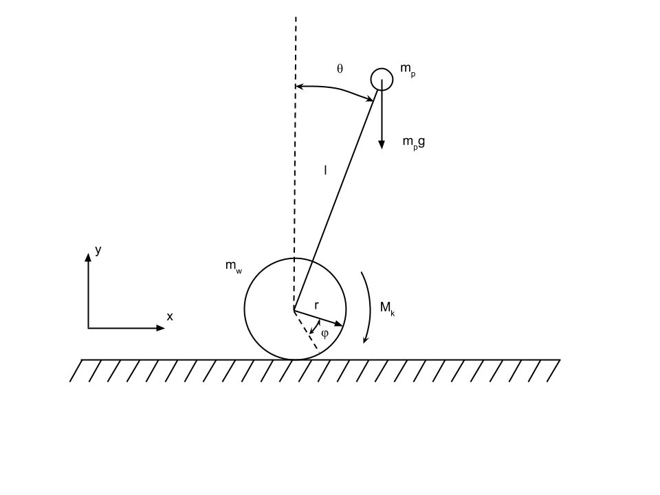
I have build my inverted pendulum robot, finally. The mathematical model and lqr redulator were build to complete the task.
Final result is shown in the video:


First of all I tried to build robot with PID control, but after multiple tries I gave up and deside to make a mathematical model and build control with it.

Mathematical model


We will consider the system consists of inverted pendulum on a wheel represented above.The friction isn't considered. Pendulum will be a point mp,fixed with weightless stick of length l to wheel. The wheel is considered a ring with radius r and mass mw. The momentum of motor will be Mk
mp: pendulum mass
mw: wheel mass
l: pendulum length
r: wheel radius
θ: angle between pendulum and vertical line
φ:angle of wheel rotation relative to it's initial position
Mk: motor momentum

For research of system we will use Euler-Lagrange's equations.
$\frac{d}{dt}(\frac{\partial L}{\partial \dot{q}}(q,\dot{q}))-\frac{\partial L}{\partial {q}}(q,\dot{q})=\tau$ (1.1)

We will express position of the center of a wheel through an angle of rotation:
$x=r \phi$ . (1.2)
We will notice that coordinates of the center of mass of a pendulum are on the following ratios:
$x_g =x +l sin (\theta)$ (1.3)
$y_g =l cos(\theta)$ (1.4)
 
At first we will calculate representation for kinetic energy of system. Kinetic
energy of a pendulum is equal
$T_p= \frac{1}{2}[m_p \dot{y}_g^2 (t )+ m_p \dot{x}_g^2(t) ]$ . (1.5)
Kinetic energy of a wheel is equal
$T_w= \frac{1}{2}[m_w \dot{x}^2 (t )+ m_w r^2 \dot{\phi}^2(t) ]$ (1.6)
Substituting (1.2), (1.3),(1.4) in (1.5) and (1.6) we will receive total kinetic energy
$T= \frac{1}{2}m_p l^2 \dot\theta sin(\theta)^2+ \frac{1}{2}m_p r^2\dot{\phi}^2+ \frac{1}{2}m_p l^2\dot{\theta}^2 cos(\theta)^2+ m_w r^2 \dot{\phi}^2+\frac{1}{2}m_p l^2 \dot{\theta}^2$ (1.7)
Total potential energy is
$\Pi =m_p g l cos (\theta)$
Lagrange's function is set on a formula $L=T-\Pi$
As a result we have
$L=\frac{1}{2}m_p l^2 \dot\theta sin(\theta)^2+ \frac{1}{2}m_p r^2\dot{\phi}^2+ \frac{1}{2}m_p l^2\dot{\theta}^2 cos(\theta)^2+ m_w r^2 \dot{\phi}^2+\frac{1}{2}m_p l^2 \dot{\theta}^2-m_p g l cos(\theta)$

We will remove the equations of the movement by means of Lagrange's equations of the second sort (1.1).
As the generalized coordinates we will take angles of rotation of a wheel and a pendulum. Then
the vector of the generalized coordinates is presented in the form
$q=\begin{pmatrix} \phi \\ \theta \end{pmatrix}$
The vector of the generalized forces looks as follows:
$\tau=\begin{pmatrix}M_k\\0\end{pmatrix}$
Having substituted (1.1) derivatives in Lagrange's equations, we receive the equations
movements:
$r cos(\theta)l m_p \ddot\theta+r^2(m_p+2m_w)\ddot\phi-rsin(\theta)\theta^2lm_p=M_k$ (1.5)
$\ddot\phi cos(\theta)l m_p r-m_p g l sin(\theta)+2m_pl^2\ddot\theta=0$ (1.6)

Let the system be represented in standart form:
$M(q)\ddot q+C(q,\dot q)\dot q+G(q)=\tau$, where
$q=\begin{pmatrix} \phi \\ \theta \end{pmatrix}$,
$M(q)=\begin{bmatrix}r^2(m_p+2m_w) & r cos(\theta)l m_p\\ r cos(\theta)l m_p & 2 m_p l^2 \end{bmatrix}$,
$C(q,\dot q)=\begin{bmatrix} 0 & -r \dot \theta sin(\theta)l m_p\\  0 & 0 \end{bmatrix}$,
$G(q)=\begin{pmatrix} 0 \\ -m_pg l sin(\theta) \end{pmatrix}$ и
$\tau=\begin{pmatrix}M_k\\0\end{pmatrix}$

For control of the received system we will construct linear quadratic regulator.
For this purpose we will carry out linearization of the received equations of the movement (1.5) and (1.6) in
vicinities of zero position of a pendulum:
$\frac{d}{dt}\begin{bmatrix} \phi \\ \dot \phi \\ \theta \\ \dot \theta\end{bmatrix}=AX+BM_k=\begin{bmatrix}0 & 1 & 0 & 0\\0 & 0 & \frac{-m_p g}{r(m_p+4m_w)} & 0\\ 0 & 0 & 0 & 1\\ 0 & 0 & \frac{g(m_p+2m_w)}{l(m_p+4m_w)} & 0 \end{bmatrix}\begin{bmatrix} \phi \\ \dot \phi \\ \theta \\ \dot \theta\end{bmatrix}+\begin{bmatrix} 0 \\ \frac{2}{r^2(m_p+4m_w)} \\ 0 \\ \frac{1}{l r (m_p+4m_w)}\end{bmatrix}M_k$

The problem of optimum control is in detail sorted in the book of professor V. N. Afanasyev "Optimum
control systems. Analytical designing". In this article I won't stop on it.

Control


I calculated control by means of MatLab, there is a lqr function which calculates coefficients.

Simulation

I made modeling in simulink and here that turned out:


Hardware implementation

For calculation of a corner data from the accelerometer and a gyroscope come to the complementary filter (RC filter).


float lastCompTime=0;
float filterAngle=1.50;
float dt=0.005;//0.002 //0.005

float comp_filter(float newAngle, float newRate) {

dt=(millis()-lastCompTime)/1000.0;
float filterTerm0;
float filterTerm1;
float filterTerm2;
float timeConstant;

timeConstant=0.5; // default 1.0

filterTerm0 = (newAngle - filterAngle) * timeConstant * timeConstant;
filterTerm2 += filterTerm0 * dt;
filterTerm1 = filterTerm2 + ((newAngle - filterAngle) * 2 * timeConstant) + newRate;
filterAngle = (filterTerm1 * dt) + filterAngle;
lastCompTime=millis();
return filterAngle;
}

On motors quadrature enkoder are established, was to use interruptions to me laziness and I copied a stanadartny code from arduino examples


void doEncoder() {
  if (digitalRead(encoder0PinA) == HIGH) {
    if (digitalRead(encoder0PinB) == LOW) {  // check channel B to see which way
                                             // encoder is turning
      encoder0Pos = encoder0Pos - 1;         // CCW
    } 
    else {
      encoder0Pos = encoder0Pos + 1;         // CW
    }
  }
  else                                        // found a high-to-low on channel A
  { 
    if (digitalRead(encoder0PinB) == LOW) {   // check channel B to see which way
                                              // encoder is turning  
      encoder0Pos = encoder0Pos + 1;          // CW
    } 
    else {
      encoder0Pos = encoder0Pos - 1;          // CCW
    }
  }
}

Further all values of sensors come to the LQR regulator:


float K1=0.1,K2=0.29,K3=6.5,K4=1.12;
long getLQRSpeed(float phi,float dphi,float angle,float dangle){
  return constrain((phi*K1+dphi*K2+K3*angle+dangle*K4)*285,-400,400);
}

And further value of the regulator arrive on motors. Unfortunately, calculated values of the regulator didn't stabilize the robot and it was necessary to correct them approximately. 

Then I added possibility of control from phone. For this purpose I connected bluetooth to pins of serial of port the HC-05 module.


float getPhiAdding(float dif){

  if(dif-200){return 0.f;}
  float ret = dif*0.08;

  return ret;
}

float getFactorAdding(float dif){
  if(dif-200){return 0.f;}
  float ret = dif/500*20;
  Serial.println(ret);
  return ret;
}
//==============================================
 if (Serial.available()){
    BluetoothData=Serial.read();
     if(BluetoothData=='w'){   
      phiDif=200;//constrain(phiDif+10,-200,200);
     } else if(BluetoothData=='s'){ 
      phiDif=-200;//constrain(phiDif-10,-200,200);      
     } else if(BluetoothData=='a'){   
      factorDif=200;//constrain(factorDif+10,-200,200);
     } else if(BluetoothData=='d'){   
      factorDif=-200;//constrain(factorDif-10,-200,200);      
     } else if(BluetoothData=='c'){   
      factorDif=0;//constrain(factorDif-10,-200,200);      
      phiDif=0;
     }
    }

encoder0Pos+=getPhiAdding(phiDif);
float factorL=getFactorAdding(factorDif);
md.setSpeeds(spd-factorL,spd+factorL);


© Alexander Semion